
Unforeseen events are a fact of life. When it comes to inventory management, safety stock helps fill the gap when cycle stock is insufficient. The task for inventory managers is to calculate the appropriate amount of safety stock so that there’s enough to cover all situations without overwhelming the storage area or working capital budget.
According to the APICS Dictionary, safety stock is inventory that is carried to protect against forecast errors, as well as fluctuations in demand or supply. This type of stock, also known as buffer stock or reserve stock, is intended to reduce the frequency of stockouts and, in turn, enable companies to provide better customer service.
Some inventory managers use rules of thumb to govern safety stock amounts, such as the guideline that safety stock levels should equal 10-20% of cycle stock or two weeks’ worth of coverage. However, determining the appropriate safety stock level should be a bit more nuanced because it depends on supply and demand variability.
Accounting for demand variability
Calculating the appropriate safety stock level in the face of variable customer demand requires some basic statistics knowledge.
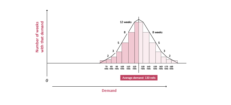
Figure 1 is a histogram, a plot showing the number of cycles at which each demand range occurs. In this case, the histogram plots demand for rolls of a specific grade of paper made on a paper-forming machine throughout 52 weeks. Actual demand was very close to the average —130 rolls per weekly production cycle — for 12 weeks of the year, when the actual demand was 125-135 rolls. Then, actual demand was 135-145 rolls for eight weeks and 145-155 rolls for five weeks. As actual demand extends higher above average, the number of weeks that actual demand was within that range decreases. There is a similar pattern on the other side of the average: Demand was 115-125 rolls for eight weeks and 105-115 rolls for five weeks. This bell-shaped curve is typical of many demand patterns.
Figure 1: An example histogram of weekly paper demand throughout 52 weeks
Some products will have little variability and thus a very narrow histogram. Others will have higher variability and a wider histogram. The width of the curve and the underlying variability can be characterized by a statistical property called standard deviation, which is symbolized by sigma. Although the calculation of standard deviation is beyond the scope of this discussion, understanding sigma can help with calculating how much safety stock is needed to provide various levels of protection against demand variability.
In this example, if the company does not have any safety stock, and only 130 rolls of cycle stock, there will be enough stock to satisfy demand during only half the cycles in the year. The company will face stockouts in the other half of the cycles.
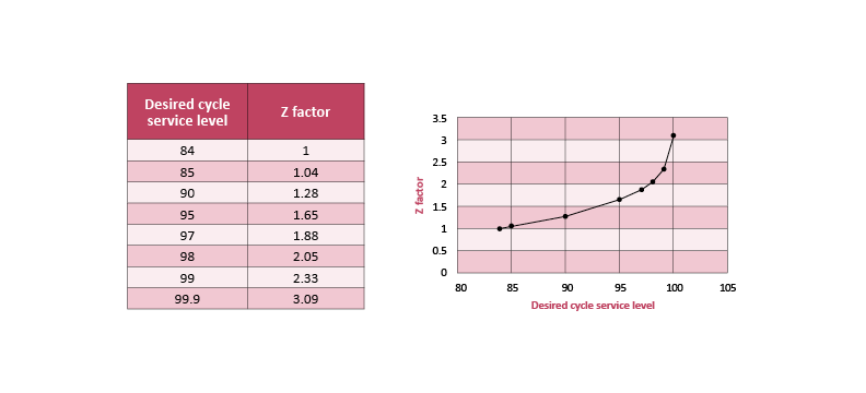
Statistics teaches that if a company carries extra stock equal to 1 sigma, that will be enough to cover demand for 84% of the cycles. Sigma is 28 rolls in this example, so if the company carries 28 rolls of safety stock in addition to the 130 rolls of cycle stock, that should be sufficient to prevent stockouts during 44 of the 52 weeks. If safety stock equals 2 sigma, that should cover 98% of the cycles.
A company’s ideal safety stock level will be based on its tolerance for stockouts. For example, if company leaders decide that the company can tolerate stockouts during no more than 2% of the cycles, that sets the cycle service level (CSL) goal at 98%, which requires 2 sigma of safety stock, or 56 rolls in this example. A CSL is the percentage of cycles in which a company hopes to not have stockouts. The number of sigma required to achieve the CSL is called the service-level factor, or Z factor.
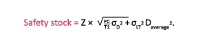
The general equation for the amount of safety stock required to cover demand variability is:

Z is the Z factor and is demand variability.
Figure 2 shows the relationship between Z and service level. The relationship is highly nonlinear: higher service-level values — or a lower potential for stockouts — require disproportionally higher safety stock levels. Statistically, a 100% service level is impossible. Typical service-level goals are in the 90%-98% range.
Good inventory management practice suggests that Z should be set independently for groups of products based on strategic importance, profit margin, dollar volume or some other criteria. This will result in more safety stock for those stock keeping units that are more valuable to the business and less safety stock for products believed to be less important to business success.
Figure 2: The relationship between service factor and service level
Watch the time units
The above equation assumes that the standard deviation of demand is calculated from a dataset in which the demand periods are equal to the lead time or production cycle length. If not, an adjustment must be made to the standard deviation value to statistically estimate what the standard deviation would be if calculated based on periods equal to the total lead time. As an example, if the standard deviation of demand is calculated from weekly demand data, and the lead time is two weeks, the standard deviation of demand calculated from a data set covering two-week periods would be the weekly standard deviation times the square root of the ratio of the time units, or
In the guide “Logistical Management,” authors Donald Bowersox and David Closs use the term performance cycle (PC) to denote the total lead time. For procuring raw materials, PC includes the time to decide what to order, communicate the order to the supplier, manufacture or process the materials, deliver them, and place them in inventory. Inside a manufacturing facility, the PC includes the time to decide what to produce, manufacture the material, release the material to the downstream inventory and return to the next cycle. In the event that a customer allows for a delivery lead time that is greater than the time needed to deliver the order, the remaining customer lead time can be subtracted from the PC.
The PC also can be considered the time at risk, such as the amount of time between the point when someone determines how much to order or produce and the point when the next determination is made and realized.
Using T1 to represent the time increments from which the standard deviation was calculated — which are one-week increments in our example — and PC to represent the total lead time or performance cycle length, this is the equation for safety stock:

Working from a forecast
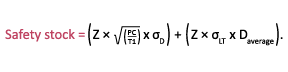
If cycle stock has been calculated from historical demand, then the variance used in the safety stock calculation should be based on past demand variation. If forecasts are used to set cycle stock, then the factor requiring protection is forecast error. Standard deviation of forecast error would replace standard deviation of past demand in the safety stock formula, which would become this equation:

It is critical that the same time units — whether days, weeks or another unit of time — are used for all variables.
If there is bias in the forecast, the forecasting process must be improved to reduce and then eliminate the bias. Forecast bias will result in underestimating or overestimating the amount of needed cycle stock.
It also should be noted that the PC/T1 factor is a statistical adjustment to approximate the standard deviation of demand throughout the time period of the performance cycle and is just an approximation. It gives reasonable results in cases when the performance cycle is greater than the data collection time period. However, it can give very poor results going in the other direction — where PC is less than T1 — especially when the time parameters are small, such as when going from weeks to days. If PC is much less than T1, it’s useful to try to measure demand variability or forecast error on a more frequent basis to reduce T1 to a frequency closer to PC. Ideally, PC equals T1 so that no adjustment is needed.
Seasonal switches
If seasonality is a significant cause of demand variability, cycle stock should be periodically adjusted to reflect the forecast demand during the various high and low periods. If seasonality is not recognized and is instead treated as normal demand variability, a company could end up having a very high level of safety stock while being unable to provide enough material to cover demand in the peak season.
Lead time variability
If lead time variability, as opposed to demand variability or forecast error, is of concern, safety stock should be calculated with this equation:

The average demand term (Daverage) is included in the equation to convert the standard deviation of the lead time, which is expressed in time units, into production in volume units, such as cases, gallons, pounds or rolls. This equation does not need an adjustment for PC.
Combining variability
If both demand variability and lead time variability are present, the safety stock required to protect against each factor can be combined statistically, which results in a lower total safety stock than the sum of the two individual calculations. If demand variability and lead time variability are independent — meaning that they are caused by different influences — and they both are reasonably normally distributed, the combined safety stock equation is as follows:
The reasoning behind this equation is that, if the two variabilities are independent, it is very unlikely that demand extremes will occur at the same time as very long lead times. Note that the demand elements are all squared, similar to the equation for the hypotenuse (C) of a right triangle with sides A and B:

If demand variability and lead time variability are not statistically independent of each other, safety stock is equal to the combination of the equations for demand variability and lead time variability:
Alternate approaches to safety stock
The calculations in this article sometimes result in safety stock recommendations that are more than businesses can afford to carry. For these situations, there are alternate approaches.
Sometimes an expediting process can be designed that can prevent a stockout when safety stock is insufficient to cover all random variation. For example, if the goal is a 98% cycle service level (CSL), safety stock can be reduced by about 38% — to a Z factor of 1.28 rather than 2.05 — if the company opts for a 90% CSL coupled with a contingency plan that prevents stockouts in the other 8% of cycles. However, the contingency plan must be planned and agreed upon in advance. It is unacceptable to ignore this step in the hopes that something can be figured out when the time comes.
This practice is especially appropriate when working with very expensive products, which are costly to carry in inventory. In one specific example involving an expensive but relatively lightweight product, total supply chain cost was reduced significantly by carrying small amounts of safety stock in overseas warehouses and then relying on air freight to cover demand peaks. The cost of air freighting a small percentage of the total demand was minimal compared with the cost of carrying large safety stocks of this highly valuable material on an ongoing basis.
Another alternative is to consider if a make-to-order (MTO) approach is possible. If lead times allow it, MTO completely eliminates the need for any safety stock — or cycle stock, for that matter. If lead time commitments will not allow for full MTO, finish-to-order (FTO) can enable a company to locate the safety stock where it is generally far less differentiated. Then demand variability will be much less, on a relative basis, and safety stock requirements will be lower than they would be with finished product inventory. Customers will sometimes be willing to accept longer lead times for highly sporadic purchases, making FTO or MTO more of a possibility.
Satisfying corporate goals
Although meeting a certain CSL is useful, business leaders often are more concerned about the percentage of total volume ordered that is available to satisfy customer demand. This is known as fill rate and often is considered to be a better measure of inventory performance. While CSL is an indication of the frequency of stockouts without regard to the total magnitude, fill rate is a measure of inventory performance on a volumetric basis.
The specific calculations of safety stock required to achieve a desired fill rate are complex and beyond the scope of this article. However, the basics of this concept still are important. With stable demand patterns and supply behavior — that is, low standard deviations of demand and lead time — fill rate will generally be higher than CSL. Although stockouts will occur, the magnitude of each stockout will be small because of the low supply and demand variability. The opposite also is true. If there is high variability in demand or lead time, the magnitude of any stockout can be quite high despite carrying safety stock. In this case, the fill rate actually is less than CSL.
Frequent stockouts leave customers in difficult situations, resulting in supply chain bottlenecks if components are unfulfilled or upset customers if there is not enough stock to meet demand. In short, it’s important to be smart about safety stock in order to keep supply chains moving.
Editor’s Note: This article is a continuation of “Better Planning and Scheduling with the Right Cycle Stock Levels” from the October-December 2020 issue. The previous article described the role of cycle stock and how to determine appropriate levels. Now, this article focuses on the important role of safety stock.