This is the third in a series of posts about operations and support for complex systems (or systems of systems), such as an electrical grid, railroad line, or assembly line. Such systems are nearly ubiquitous in business today, but we rarely consider their supply chain requirements until there is a problem.

Effectively managing a system’s operations and support (O&S) costs while also achieving and sustaining a desired operational performance target requires a careful balance between inputs and outputs. This is best accomplished when managers employ a systems-level perspective.

As we learned in our last post, analytical optimization techniques, like readiness-based sparing (RBS) models, can help quantify the relative contribution of each logistics resource toward overall capability and performance. Unfortunately, such optimization tools have a very structured view of a system’s operation and performance. Therefore, managers need a more comprehensive approach to understand the operations and performance of complex systems with multiple, interrelated subsystems. Modern simulation tools can fulfill that requirement and assess the contribution and robustness of multiple logistics capabilities—including inventory, maintenance, and distribution systems—within a system of systems context.

To guide complex systems toward a desired system-level performance, managers must be able to rightsize their resource inputs. Rightsizing involves more than identifying the capacity of key logistics factors. To adequately rightsize O&S inputs, managers must consider how to best apply resources to address a particular task. They also must contemplate various levels of uncertainty when deciding where to deploy resources.

Models help us contend with uncertainty in decision making. They offer useful insights into a system’s likely behavior under a range of conditions by allowing us to look at the inherent characteristics of a system and understand the system’s tendency to respond to any number of external disturbances.

For example, suppose a particular aircraft maintenance action needs 10 parts. If nine of those parts are issued from supply for a 90 percent fill rate, that’s pretty good, right? Unfortunately, if the missing 10th part is critical to completing the repair, but it is on backorder, then the supply issue can ground the aircraft and perhaps jeopardize an airline’s scheduled performance. With models, we can play out this scenario and gauge its effect on the system as a whole.

Let’s look at two specific aspects of logistics modeling: Monte Carlo simulations and Stochastic Petri nets (SPNs). A Monte Carlo simulation is a modeling technique for quantifying how a system is likely to behave under uncertainty. This type of simulation relies on many replications of probabilistically generated process activities and durations to achieve a statistical level of confidence in the predicted performance outcomes.

An example might be modeling how long it takes a fleet of snowplows to clear a city’s streets after a snowfall. The amount of snow and ice (a probabilistic variable) affects how quickly each snowplow can clear its assigned route (another probabilistic variable). The aggregate operating hours for the snowplow fleet, in turn, can influence likely vehicle failures (also probabilistic) and resultant demands upon supply and maintenance activities. Playing out this scenario many times, using different random number streams to interject the effects of variability, allows us to ultimately develop a statistically robust estimate of each likely probabilistic outcome.

SPNs are a class of network-oriented, Monte Carlo–capable simulation models. Within an SPN, there are three key components:

• Entities (or objects) perform activities.
• Places represent an entity’s physical state.
• Connections are transitional paths that entities follow as their physical state changes over time.

Petri nets explicitly allow for time-varying entity characteristics, such as aging components and their associated performance deterioration. Petri nets also offer a way to visualize system and subsystem capability so that managers can see where bottlenecks occur or where slack capacity exists.

Figure 1 is an SPN simulation of an unmanned aerial vehicle (UAV) mission. Aircraft are selected from an available pool and monitored through a preflight check and take-off. After transiting to the orbit area, the surveillance mission begins. At some point, the UAV must call for a relief aircraft to continue the surveillance. After the original aircraft departs the mission area, it returns to base for a post-flight check and any requisite corrective maintenance. Supporting this mission are the line-of-sight (LOS) ground-based subsystems, which must be fully operational for UAVs to take off and land. During the simulation’s animation, colors are used to reflect an entity’s condition: Blue items are available, green ones are performing their missions, and red ones are unserviceable.

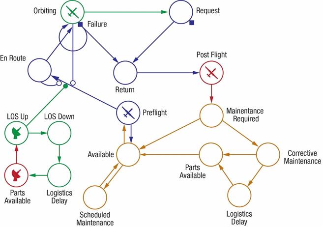
_{Figure 1: A sample simulation network for a UAV mission using Stochastic Petri nets} 

In this simulation, coverage statistics about the percent of time a UAV is in orbit are collected. Because SPN transitions incorporate probabilistic attributes, an SPN simulation played out through many replications can statistically describe the likely performance of logistics decisions when systems operate in uncertain conditions, such as during a supply chain disruption or a surge in operational intensity.

Although the example in Figure 1 is simplified, it retains a relevant level of detail for decision making. And that is the beauty of a Petri net: its flexible, yet transparent portrayal of any number of subsystem entities, places, and connections.

Simulations like these allow managers of complex systems to evaluate analytically optimal O&S decisions by implementing them in a virtual environment, stress-testing the decisions, and then statistically quantifying the overall system’s resilience to uncertainty.

Such simulations also allow system managers to isolate a particular logistics resource in order to examine its relative contribution to the system’s overall performance. Managers can then fine-tune analytically recommended logistics decisions and deployments and quickly and appropriately realign resources in response to an unforeseen event.